

When working on classification problems in Machine Learning, there are a number of useful evaluation metrics like accuracy, precision, recall, AUC/ROC, etc. Here are the mathematical forumula for these metrics:
\[Precision = \frac{TP}{TP + FP} \]
\[Recall (TPR) = \frac{TP}{TP + FN}\]
\[Accuracy = \frac{TP + TN}{TP + TN + FP + FN} \]
\[Fall Out (FPR) = \frac{FP}{TN + FP} \]
- TP = True Positives, i.e., the number of positive instances classified as positive.
- TN = True Negatives, i.e., the number of negative instances classified as negative.
- FP = False Positives, i.e., the number of negative instances mis-classified as positive.
- FN = False Negatives, i.e., the number of positive instances mis-classified as negative.
I don't know about you, but I have a hard time remembering these formulae. Being more of a visual learner, I really loved the graphic on Wikipedia, but it does not visualize all the different metrics. So inspired by that graphic, I made some of my own.
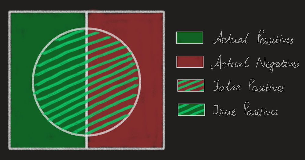
In the picture above, the rectangle is the entire dataset. The solid green side are all positive instances and the solid red side are all the negative instances. The circle is the set that was classified as positive, correspondingly everything outside the circle was classified as negative. While the above picture does not show False Negatives and True Negatives, it is easy enough to see that False Negatives are represented by the solid green part that is outside the circle, and that True Negatives are the solid red part that is outside the circle.
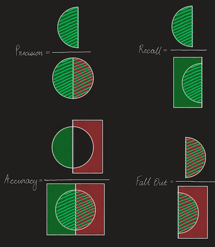
Here are the above formula in pictures -
AUC/ROC
There are a number of good blog posts that explain Area Under the Curve and Receiver Operator Characteristics, but somehow they never gave me the complete picture. So here is my own explanation:
AUC is a single metric that represents the "quality" of a classifier. There are two concepts in AUC that go hand-in-hand. One is the concept of a classifier which here is a system that given an instance will output the probability that it is positive. The second concept is that of a threshold which is used by the final application. The final application gets an instance along with the positive probability. It then applies the threshold, if the probability is above that threshold, the instance is classified as positive otherwise it is classified as negative. As can be seen in the illustrations below, the same classifier can result in different classifications depending on which threshold is used.
I like to think of AUC as a metric that takes away the effect of the threshold and tries to tell us whether the pure probabilities outputted by the classifier are good or not.
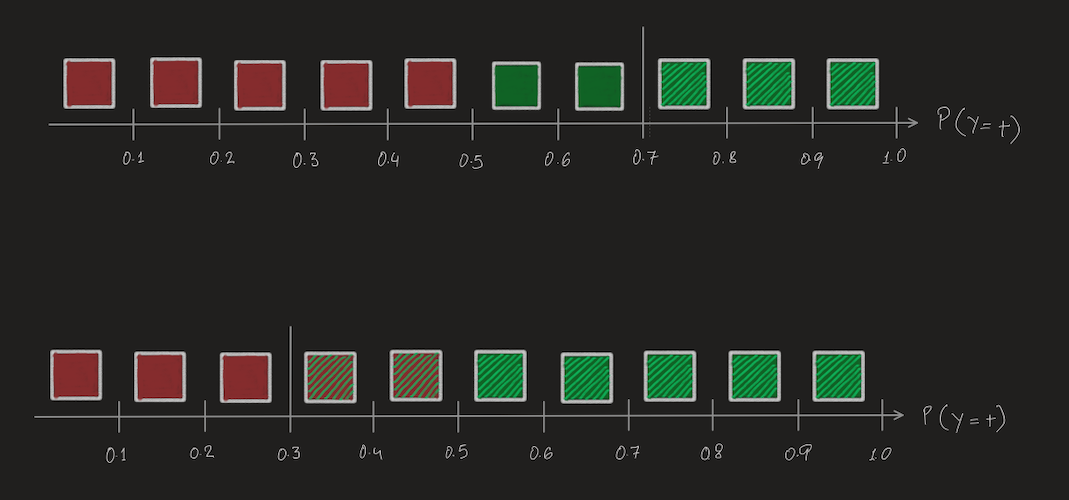
The horizontal line represents the probability with which the classifier thinks an instance is positive or negative. The solid red and green boxes represent "positive" and "negative" instances. This is a pretty good classifier, all the negative instances have lower probabilities and all the positive instances have higher probailities. But there are some instances that it is not too sure of so they are hovering around 0.5.
In the first illustration, a high threshold of 0.7 is chosen, so everything that has a probability greater than 0.7 is classified as positive, represented by the slanted bright green lines. Everything lower than 0.7 is classified as negative. In the second illustration, a low threshold of 0.3 is chosen resulting in different final classifications.
Lets calculate all the metrics for both the thresholds -
For threshold of 0.7
\[Accuracy = \frac{8}{10} = 0.8\]
\[Precision = \frac33 = 1 \]
\[Recall (TPR) = \frac35 = 0.6\]
\[Fall Out (FPR) = 0 \]
For threshold of 0.3
\[Accuracy = \frac{5+3}{10} = \frac{8}{10} = 0.8\]
\[Precision = \frac57 = 0.71\]
\[Recall (TPR) = \frac55 = 1\]
\[Fall Out (FPR) = \frac25 = 0.4\]
If we keep increasing the threshold the FPR remains 0, but the TPR will keep decreasing. On the other hand, if we keep decreasing the threshold, the FPR will keep increasing, but the TPR will remain at 1.
For AUC we just need the TPR and FPR. Both these thresholds gave us two points on the AUC curve for this particular classifier - (0, 0.6) and (0.4, 1). The complete AUC curve for this classifier is built from computing the TPR and FPR for a lot of different thresholds. The area under this curve is then called the AUC for this classifier. This single number is then taken as a measure of quality for this classifier. For a different classifer, the TPR and FPR are evaluated for a bunch of thresholds and the curve plotted with these values resulting in a different AUC.
Photo by Scott Webb on Unsplash